Microring Resonator
Introduction
 Microring resonator is important filtering device in photonic integrated circuits, the high performance filter require a wide free spectrum range(FSR) and high quality factor. Obtaining a large spectral range for microring resonator requires the use of a small radius, but too small radius can cause bending loss and reduce the quality factor. In order to meet the requirements of wide free spectrum range and high quality factor, it is necessary to carefully design the size of the ring and coupling efficiency.
In this example, we demonstrate the use of finite difference eigenmode(FDE) solver to calculate the group refractive index of an optical waveguide, then calculate the effective refractive index of symmetric and anti symmetric modes at the coupling region between the straight waveguide and the ring, and finally use 3D FDTD simulation to calculate the transmittance of the drop port.
Simulation
1 Code Description
1.1 Import Toolkit
First, we need to import "maxoptics_sdk" and third-party package of Python. The import module for FDE and FDTD simulation as follows.
from typing import List, Literal, NamedTuple
import time
import maxoptics_sdk.all as mo
from maxoptics_sdk.helper import timed, with_path
1.2 Define Simulation Function and parameters
To facilitate parameter changes, we can define function to encapsulate the entire simulation project. Before starting the simulation, you can define variables to control the parameters. As shown below.
def simulation(*, wavelength, grid, number_of_trial_modes, run_options: "RunOptions", **kwargs):
# region --- 0. General Parameters ---
width = 0.4
radius = 2.8
waveform_name = f"wv{wavelength*1e3}"

path = kwargs["path"]
simu_name = f"Microring_resonator"
time_str = time.strftime("%Y%m%d_%H%M%S", time.localtime())
project_name = f"{simu_name}_local_{time_str}"
plot_path = f"{path}/plots/{project_name}/"
kL = [f"0{k}" for k in range(5)]
export_options = {"export_csv": True, "export_mat": True, "export_zbf": True}
# endregion
1.3 Create project
We create an empty project by instantiating "Project()" in the simulation environment and define the name of project.
# region --- 1. Project ---
pj = mo.Project(name=project_name)
# endregion
1.4 Add Material
Here we demonstrate using "Material()" to instance the material module into the project, "add_nondispersion" and "add_lib" functions are available to create materials. You can refer to the following script to set materials.
# region --- 2. Material ---
mt = pj.Material()
mt.add_lib(name="Si", data=mo.Material.Si_Palik, order=2)
mt.add_lib(name="SiO2", data=mo.Material.SiO2_Palik, order=2)
# endregion
The "name" defines the name of the added material.
The "data" specifies the real and imaginary parts of the refractive index of the material.
The "order" specifies the mesh order of the material.
1.5 Add waveform
Adding a light source for simulating in 3D FDTD, and we use Waveform to set the waveform parameters of the light source.
# region --- 3. Waveform ---
wv = pj.Waveform()
wv.add(name=waveform_name, type='gaussian_waveform',
        property={'set': 'frequency_wavelength',  # selections are ['frequency_wavelength','time_domain']
                    'set_frequency_wavelength': {
                        'range_type': 'wavelength',  # selections are ['frequency','wavelength']
                        'range_limit': 'center_span',  # selections are ['min_max','center_span']
                        'wavelength_center': wavelength,
                        'wavelength_span': 0.1,},
                    }
        )
wv_id = wv[waveform_name]
# endregion
The "name" sets the name of the waveform.
The "wavelength_center" sets the center wavelength of the light source.
The "wavelength_span" sets the wavelength range of the light source.
1.6 Add Structure
# region --- 4. Structure ---
st = pj.Structure()

st.add_geometry(name="ring", type="Ring",
                property={ "geometry": { "x": 0, "y": 0, "z": 0, "z_span": 0.22,
                                        "inner_radius": radius - width/2, "outer_radius": radius + width/2},
                            "material": {"material": mt["Si"], "mesh_order": 3 }})
st.add_geometry(name="wg_1", type="Rectangle",
                property={"geometry": {"x": 0, "x_span": 15, "y": 3.3, "y_span": width, "z": 0, "z_span": 0.22},
                            "material": {"material": mt["Si"], "mesh_order": 3}})
st.add_geometry(name="wg_2", type="Rectangle",
                property={"geometry": {"x": 0, "x_span": 15, "y": -3.3, "y_span": width, "z": 0, "z_span": 0.22},
                            "material": {"material": mt["Si"], "mesh_order": 3}})
# endregion
| Key | Value | Type | Description |
|---|---|---|---|
| x | 0 | float | center position in the x-direction of the geometric structure |
| material | mt["Si"] | material | select the material added Materials |
| mesh_order | 3 | integer | set the priority of the material |
| x | 0 | float | the center coordinate of the ring in the x-direction |
| y | 0 | float | the center coordinate of the ring in the y-direction |
| z | 0 | float | the center coordinate of the ring in the z-direction |
| z_span | 0 | float | the thickness of the ring in the z-direction |
| inner_radius | 2.6 | float | the size of the inner radius of the ring |
| outer_radius | 3 | float | the size of the outer radius of the ring |
The properties of the ring structure are shown in the table above, properties of Rectangle can refer to the settings of the ring. Select simulation material by using mesh_order in areas where geometry overlaps, the priority of structural materials needs to be higher than that of background material.
1.9 Add Solver
# region --- 7. Simulation
simu = pj.Simulation()
simu.add(name=simu_name, type="FDTD",
            property={"background_material": mt["SiO2"],
                    "geometry": {"x": 0, "x_span": 9, "y": 0, "y_span": 9, "z": 0, "z_span": 2},
                    "boundary_conditions": {
                    "x_min_bc": "PML", "x_max_bc": "PML", "y_min_bc": "PML", "y_max_bc": "PML", "z_min_bc": "PML", "z_max_bc": "PML",
                    "pml_settings": {"all_pml": {"layers": 8, "kappa": 2, "sigma": 0.8, "polynomial": 3, "alpha": 0, "alpha_polynomial": 1}}},
                    "general": {"simulation_time": 4000},
                    "mesh_settings": {"mesh_factor": 1.2, "mesh_type": "auto_non_uniform",
                                    "mesh_accuracy": {"cells_per_wavelength": grids_per_lambda},
                                    "minimum_mesh_step_settings": {"min_mesh_step": 1e-4},
                                    "mesh_refinement": {"mesh_refinement": "curve_mesh"}},
                    "advanced_options": {"auto_shutoff": {"auto_shutoff_min": 1.00e-4, "down_sample_time": 200}},
                })
# endregion
The properties settings for the FDE solver as follows.
| Key | Value | Type | Description |
|---|---|---|---|
| solver_type | 2d_x_normal | string | select the solution plane |
| dy | grid | float | grid size along the y-direction |
| dz | grid | float | grid size along the z-direction |
| calculate_modes | run_options.run_fde | bool | choose whether to calculate the mode of the waveguide |
| mesh_structure | False | bool | choose whether to calculate the refractive index distribution of the structure |
| wavelength | wavelength | float | calculate the wavelength of the mode |
| number_of_trial_modes | number_of_trial_modes | integer | number of solving modes |
| search | max_index | string | choose "max_index" or "near_n" for finding modes |
| calculate_group_index | True | bool | choose whether to calculate the group refractive index |
The properties settings for the FDTD solver as follows.
| Key | Value | Type | Description |
|---|---|---|---|
| simulation_time | 5000 | float | set the maximum simulation time |
| mesh_type | auto_non_uniform | string | select 'auto_non_uniform' or 'uniform' to set the type of grid |
| cells_per_wavelength | grids_per_lambda | integer | set the size of the grid |
| min_mesh_step | 1e-4 | float | set the minimum grid size |
| auto_shutoff_min | 1.e-4 | float | set the energy threshold for terminating the simulation |
| down_sample_time | 200 | float | set additional simulation duration |
| thread | 4 | integer | number of threads allocated to run the program |
In the settings of the FDE solver, use "calculatemodes" controls whether to calculate the mode. Note that we need to calculate the group refractive index of the waveguide, so set the "calculate group_index" to True.
In the setting of the FDTD solver, "simulation_time" is used to control the simulation time. We set the simulation time to 4000 fs, which is greater than the default value of 1000 fs. The micro ring resonator has a high quality factor, its simulation requires longer time. If the simulation time is set too small and the simulation stops before the field decays, the results obtained are incorrect.
1.8 Add FDTD Port
In the FDTD simulation, at least a light source is required. We use the "Port()" to instance the port object into the project and the "add" function to add FDTD ports for the simulation. A port can serve not only as a source but also as a monitor. If there are multiple ports, it is necessary to specify which port is the source in the port group. The settings for the FDTD ports as follows.
# region --- 6. Source ---
pt = pj.Port(property={"waveform_id": wv_struct, "source_port": "port_1","monitor_frequency_points":9})

pt.add(name="port_1", type="fdtd_port",
        property={"geometry": {"x": -4.25, "x_span": 0, "y": 3.3, "y_span": 2.5, "z": 0, "z_span": 2},
                    "modal_properties": {"general": {"inject_axis": "x_axis", "direction": "forward", "mode_selection": "fundamental"}}})
pt.add(name="port_2", type="fdtd_port",
        property={"geometry": {"x": -4.25, "x_span": 0, "y": -3.3, "y_span": 2.5, "z": 0, "z_span": 2},
                    "modal_properties": {"general": {"inject_axis": "x_axis", "direction": "forward", "mode_selection": "fundamental"}}})
pt.add(name="port_3", type="fdtd_port",
        property={"geometry": {"x": 4.25, "x_span": 0, "y": 3.3, "y_span": 2.5, "z": 0, "z_span": 2},
                    "modal_properties": {"general": {"inject_axis": "x_axis", "direction": "backward", "mode_selection": "fundamental"}}})
pt.add(name="port_4", type="fdtd_port",
        property={"geometry": {"x": 4.25, "x_span": 0, "y": -3.3, "y_span": 2.5, "z": 0, "z_span": 2},
                    "modal_properties": {"general": {"inject_axis": "x_axis", "direction": "backward", "mode_selection": "fundamental"}}})
# endregion
endregion
1.10 Add Monitor
We use the "Monitor()" to instance the monitor object into the project and the "add" function to add monitors. The port can automatically calculate the transmittance and field profile of the cross-section. In time-domain simulation, it is necessary to add a time monitor at the end of the simulation to check the field strength to judge the accuracy of the simulation results.
# region --- 8. Monitor ---
""" 6.0 GlobalMonitor """
mn = pj.Monitor()
mn.add(name="Global Option", type="global_option", property={
        "frequency_power": {  # "sample_spacing": "uniform", "use_wavelength_spacing": True, ["min_max","center_span"]
            "spacing_type": "wavelength", "spacing_limit": "center_span", "wavelength_center": wavelength, "wavelength_span": 0.1, "frequency_points": 11 } }, )
mn.add(name="time_monitor_point", type="time_monitor",
        property={ "general": { "stop_method": "end_of_simulation", "start_time": 0, "stop_time": 100, "number_of_snapshots": 0 },
        "geometry": { "monitor_type": "point", "x": 0, "x_span": 0, "y": 2.8, "y_span": 0, "z": 0, "z_span": 0 },
        "advanced": {"sampling_rate": {"min_sampling_per_cycle": 10}}})

mn.add(name="z_normal", type="power_monitor",
        property={ "general": {
            "frequency_profile": { "wavelength_center": wavelength, "wavelength_span": 0.1, "frequency_points": 11}},
            "geometry": { "monitor_type": "2d_z_normal",
                            "x": 0, "x_span": 9, "y": 0, "y_span": 9, "z": 0, "z_span": 0 } })
#endregion
1.11 View Structure
You can use the "structure_show" function to view the top view of the structure, or use the "show3d()" call gui to check simulation settings.
# region --- 9. Structure Show ---
st.structure_show(fig_type="png", show=False, savepath=f"{plot_path}00_{simu_name}")
# simu[simu_name].show3d()
# endregion
1.12 Run
Pass in the name of the simulation and use "run" function to run the simulation.
# region --- 10. Run ---
eme_res = simu[simu_name].run()
# endregion
1.13 Run and Extract Results
# region --- 11. See Results ---
if run_options.extract:

    if run_options.run_fde:
        k = kL[1]
        res = results.extract(data="calculate_modes", savepath=f"{plot_path}{k}_neff_table", export_csv=True)
        print(res.to_string(index=False))
        for m in range(len(res)):
            k = kL[2]
            results.extract(data="calculate_modes", savepath=f"{plot_path}{k}_mode{m}",
                                attribute="Ey", mode=m, real=True, imag=False, **export_options, show=False)

    if run_options.run_fdtd:

        """ 01_time monitor """
        fdtd_res.extract(data='fdtd:time_monitor', savepath=f"{plot_path}{kL[1]}_TransVstime",
                         monitor_name='time_monitor_point', target='line', attribute='E',plot_x='time', real=True,
                         imag=True, export_csv=True, show=False)

        """ 02_top_profile """
        fdtd_res.extract(data="fdtd:power_monitor", savepath=f"{plot_path}{kL[2]}_profile", monitor_name="z_normal",
                            target="intensity", attribute="E", wavelength=f"{wavelength}",  export_csv=True)

        """ 03port1_modeprofile """
        fdtd_res.extract(data="fdtd:port_mode_info", savepath=f"{plot_path}{kL[3]}_port_1_profile",
                            target="intensity", attribute="E", port_name="port_1", mode=0, export_csv=True)

        """ 031_port1_Lambda_power """
        fdtd_res.extract(data="fdtd:power_monitor", savepath=f"{plot_path}{kL[3]}_port_1_T",
                            target="line", attribute="T", port_name="port_1", plot_x="wavelength", export_csv=True)

        """ 032_port2_Lambda_power """
        fdtd_res.extract(data="fdtd:power_monitor", savepath=f"{plot_path}{kL[3]}_port_2_T",
                            target="line", attribute="T", port_name="port_2", plot_x="wavelength", export_csv=True)

        """ 033_port3_Lambda_power """
        fdtd_res.extract(data="fdtd:power_monitor", savepath=f"{plot_path}{kL[3]}_port_3_T",
                            target="line", attribute="T", port_name="port_3", plot_x="wavelength", export_csv=True)

        """ 034_port4_Lambda_power """
        fdtd_res.extract(data="fdtd:power_monitor", savepath=f"{plot_path}{kL[3]}_port_4_T",
                            target="line", attribute="T", port_name="port_4", plot_x="wavelength", export_csv=True)

# endregion
1.14 Control Switch
We can control the operation of the simulation by passing in bool values through tuple, as shown in the following code. In each simulation, only one solver will be enabled. When using the FDE solver, set "run_fde" to True and "run_fdtd" to False; When using the FDTD solver, set "run_fdtd" to True and "run_fde" to False.
class RunOptions(NamedTuple):
    index_preview: bool
    run_fde: bool
    run_fdtd: bool
    extract: bool

if __name__ == "__main__":
        simulation(wavelength=1.55, grids_per_lambda=6, run_options=RunOptions(index_preview=False, run=True, extract=True))
2. Output results
Length of ring
The light traveling in the waveguide generates evanescent field on its surface, so energy couples into a nearby waveguide as the waveguide approaches. We design a microring resonant filter with an FSR of 30nm, and we can calculate the effective circumference of the microring according to the following formula. The FDE solver can be used to calculate the group refractive index of the waveguide. The following table shows the group refractive index of the waveguide cross-section in the first three modes with a wavelength of 1.55um.
| order | TEratio | neff_real | neff_imag | ng_real | ng_imag | wavelength_nm | loss_dBpcm |
|---|---|---|---|---|---|---|---|
| 0 | 0.966627 | 2.227503 | 0.0 | 4.434594 | 0.0 | 1550.0 | 0 |
| 1 | 0.046759 | 1.692711 | 0.0 | 3.467810 | 0.0 | 1550.0 | 0 |
| 2 | 0.599748 | 1.430406 | 0.0 | 1.683888 | 0.0 | 1550.0 | 0 |
Considering the transmission of the fundamental mode of TE polarization, a group refractive index of 4.43 can be obtained. Therefore, selecting a ring with an effective radius of 2.87um can meet the free spectrum range of 30nm.
Couple gap and length
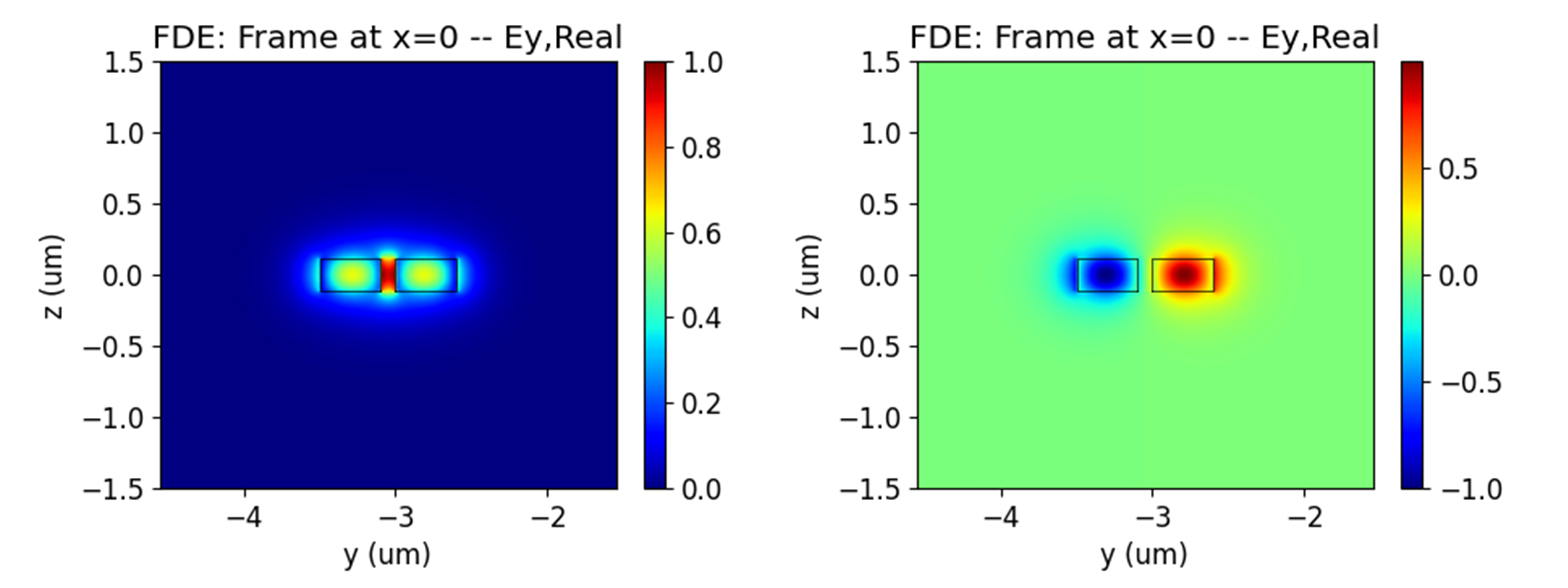
The length of the coupling region can be calculated based on the effective refractive index difference between symmetric and antisymmetric modes, as shown in the following formula. Setting the gap between the straight waveguide and the ring to 100nm can generate strong mutual coupling. Using the FDE solver to calculate the effective refractive index of the coupling region between the waveguide and the microring, the corresponding mode distribution is as follows.

The coupling distance calculated at wavelength of 1.55um more than 1.4 um. You can choose to increase the radius of the ring to reduce the coupling length. We choose to set the coupling length to zero and obtain sufficient coupling length and expected loop length by increasing the radius.
Transmission
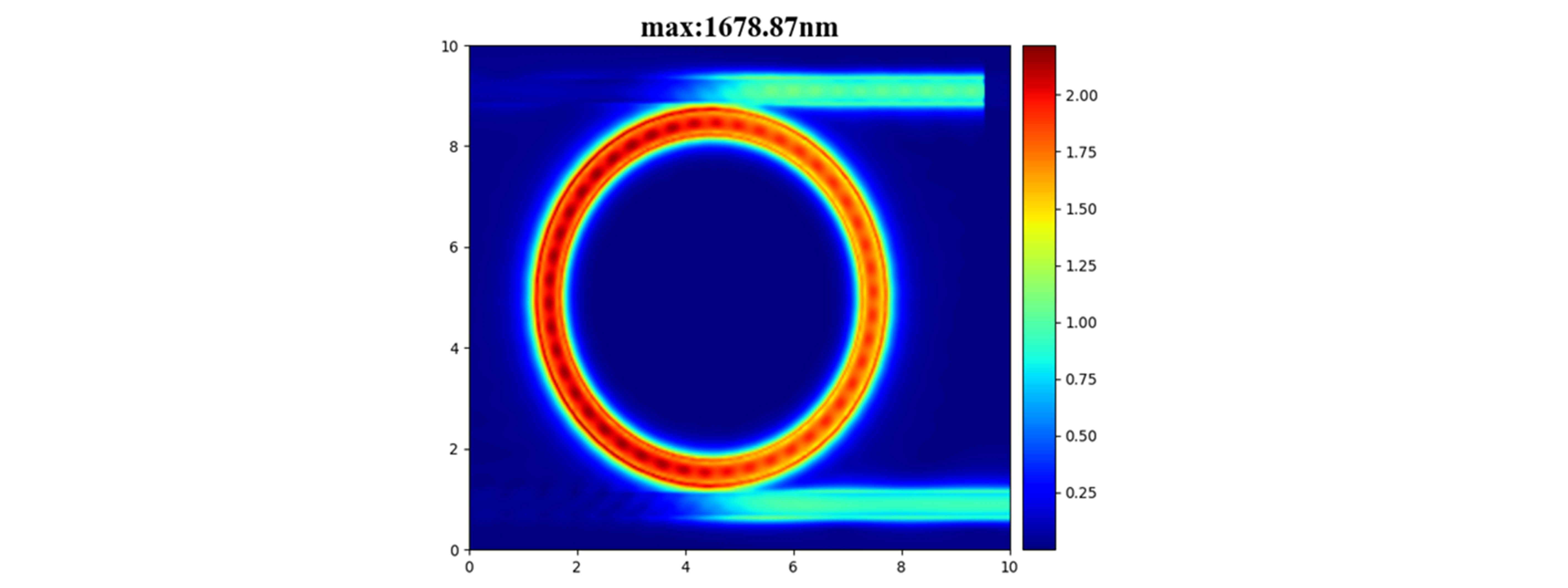
Calculate the resonant response of a straight waveguide coupled to a microring with a radius of 2.8um using 3D FDTD. Adding a mode light source as an excitation for straight waveguide, and use a power monitor to view the field distribution and transmittance.
When the light field coupled into the microring meets the resonance condition, it will output from the dorp port. As shown in the figure below, there is the maximum electric field at the drop port at the resonant wavelength.

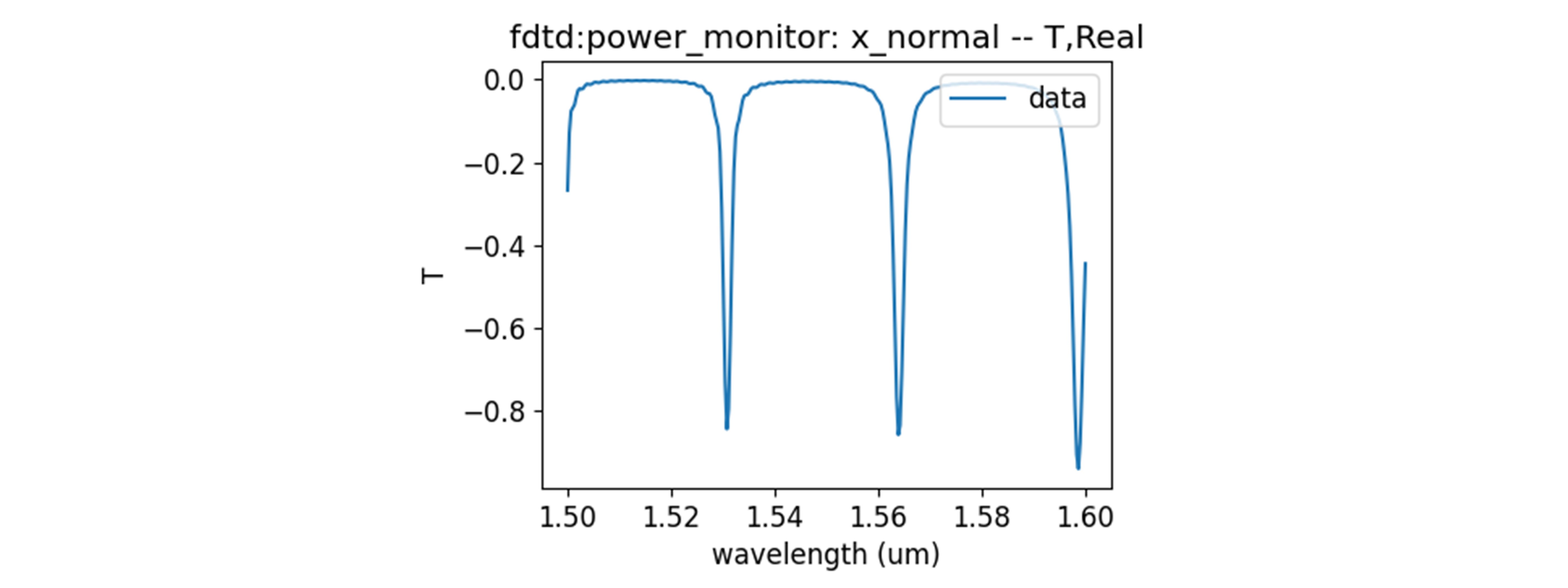
The transmittance of the drop end is shown in the following figure.

References
Hammer, M. and Hiremath, K.R. and Stoffer, R. (2004) Analytical approaches to the description of optical microresonator devices. (Invited) In: Microresonators as Building Blocks for VLSI Photonics, 18-25 October 2003, Erice, Italy. pp. 48-71. AIP Conference Proceedings 709. Springer. ISSN 0094-243X ISBN 978-0-7354-0184-6.