Y branch

Introduction

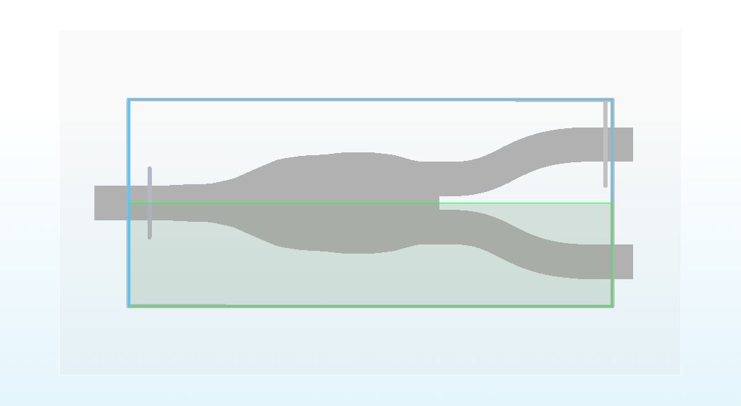
The Y branch is a fundamental component of integrated optics. Its primary function is to split the incoming light from a single input waveguide into two separate waveguides (splitter). Likewise, it can also combine light from two waveguides into a single waveguide (combiner).

The main performance parameters of the Y branch include insertion loss, device dimensions, and operating bandwidth.

Simulation Methods

Through the FDTD module or EME module, the Y branch's structure can be optimized to obtain the transmittance of fundamental mode or S-parameters of each output port. This allows the verification of the optimized results for the multi-mode interferometer.This optimization process aims to improve the Y branch's insertion loss and bandwidth performance.

Y branch(FDTD module)

1. Basic Operations

1.1 Import File

Once you have installed and configured the environment, import the python code and the GDS layout. The example library and related model code are usually located in the directory :examples/func_demo. The GDS file is generally imported into the path :examples/examples_gds

1.2 SDK Initialization

Create a new terminal and run the code after you import the python script and GDS file. Max-Optics SDK may take some time to connect the service.

2.Code Description

Now let's learn the meaning of functions and parameters that correspond to the code.

2.1 import Modules

To begin, we need to use the import command to call the relevant functional modules. For instance, we import the typing , os and time module in python. At the same time ,we import the customized module maxoptics_sdk.all and maxoptics_sdk.helper.

import maxoptics_sdk.all as mo
from maxoptics_sdk.helper import timed, with_path
import os
import time
import json
from typing import NamedTuple

The maxoptics_sdk package provides all in one optical simulation with Python.
The os module provides a way to use operating system-dependent functionality such as reading or writing to the file system, working with environment variables, and executing system commands.
The time module provides various functions to work with time-related operations and to measure time intervals.
The typing module provides support for type hints and annotations, which are used to indicate the expected types of variables, function arguments, and return values in your code.

2.2 Define Simulation

Firstly, We define parameters and give them a default value, such as the simulation wavelength and number of modes. Note that we can override this value in the following code.

@timed
@with_path
def simulation(*, wavelength=1.575,grids_per_lambda=25,run_options: 'RunOptions',**kwargs):

The provided code contains comments that define the simulation parameters. Let's explain each of these parameters.
The function simulation is used to define the simulation parameters for the program.
The wavelength parameter specifies the wavelength of the input light in micrometers.
The grids_per_lambda parameter sets the simulation mesh grid.
The **kwargs is a special syntax used in function definitions to accept an arbitrary number of keyword arguments as a dictionary.

2.3 Define Parameters

Define commonly used parameters, such as the mesh grid of the simulation boundary, the start time of the simulation, the path and name for the simulation output, the path to the imported GDS layout, and other parameters required for structural parameterized modeling.

If you need to calculate the bandwith of the device in the EME simulation, you can also decide the wavelength for sweeping in this section.

# region --- General Parameters --
waveform_name = f'wv{wavelength * 1e3}'
path = kwargs['path']
simu_name = 'FDTD_y_branch'
time_str = time.strftime('%Y%m%d_%H%M%S', time.localtime())
project_name = f'{simu_name}_{time_str}'
plot_path = f'{path}/plots/{project_name}/'
gds_file_root_path = os.path.abspath(os.path.join(path, '..'))
gds_file = gds_file_root_path + '/examples_gds/ybranch.gds'
# endregion

The code defines several parameters and variables necessary for the simulation process. The waveform_name parameter is the name of waveform.
The path variable defines the file path for the simulation, while simu_name specifies the name of the simulation file.
The time_str variable is used to obtain the current time as a timestamp for the simulation.
The project_name variable assigns a name to the project for the simulation output.
The plot_path variable determines the directory where the simulation result plots will be saved.
The gds_file_root_path and gds_file variable defines the path for importing the GDS layout.

2.4 Creat Project

You can create a new project using the Project function of Max's software development toolkit.

# region --- Project ---
pj = mo.Project(name=project_name)
# endregion

2.5 Define Materials

Let's proceed to the next step, where we set up the materials required for the simulation. In this case, we will directly use relevant materials from the MO material library.

# region --- Material ---
mt = pj.Material()
mt.add_lib(name='Si', data=mo.Material.Si_Palik, order=2)
mt.add_lib(name='SiO2', data=mo.Material.SiO2_Palik, order=2)
mt.add_lib(name='Air', data=mo.Material.Air, order=2)
# endregion

The add_lib contains three parameters name,data and order.
The data calls up the property of simulation materials in the MO material library.
The Order parameter determines the mesh order for the material during the simulation.

2.6 Waveform

In this section, we will define the property of wave.

# region --- Waveform ---
wv = pj.Waveform()
wv.add(name=waveform_name,type='gaussian_waveform',
        property={'set': 'frequency_wavelength',  # selections are ['frequency_wavelength','time_domain']
                    'set_frequency_wavelength': {
                        'range_type': 'wavelength',  # selections are ['frequency','wavelength']
                        'range_limit': 'center_span',  # selections are ['min_max','center_span']
                        'wavelength_center': wavelength,
                        'wavelength_span': 0.15,},})
wv_struct = wv[waveform_name]
# endregion

2.7 Create Model

Next, we will create the structure of Y branch.

# region --- Structure ---
st = pj.Structure()
st.add_geometry(name='in', type='Rectangle',
                property={'geometry': {'x': -1.5, 'x_span': 1, 'y': 0, 'y_span': 0.5, 'z': 0, 'z_span': 0.22},
                            'material': {'material': mt['Si'], 'mesh_order': 2}})
st.add_geometry(name="gds_file", type="gds_file",
                property={"material": {"material": mt["Si"], "mesh_order": 2},
                            "geometry": {"x": 1, "y": 0, "z": 0, "z_span": 0.22},
                            "general": {"path": gds_file, "cell_name": "splitter1", "layer_name": (0, 0)}})
st.add_geometry(name='out_up', type='Rectangle',
                property={'geometry': {'x': 3.1, 'x_span': 0.2, 'y': 0.35, 'y_span': 0.5, 'z': 0, 'z_span': 0.22},
                            'material': {'material': mt['Si'], 'mesh_order': 2}})
st.add_geometry(name='out_down', type='Rectangle',
                property={'geometry': {'x': 3.1, 'x_span': 0.2, 'y': -0.35, 'y_span': 0.5, 'z': 0, 'z_span': 0.22},
                            'material': {'material': mt['Si'], 'mesh_order': 2}})
st.add_geometry(name="waveguide_up", type="BezierWaveguide",
                property={"material": {"material": mt["Si"], "mesh_order": 2},
                            "geometry": {"x": 0, "y": 0, "z": 0, "z_span": 0.22, "width": 0.5,
                            "control_points":[{"x": 3.2, "y": 0.35}, {"x": 4, "y": 0.35}, {"x": 4, "y": 0.85},{"x": 5.2, "y": 0.85}]}})
st.add_geometry(name="waveguide_down", type="BezierWaveguide",
                property={"material": {"material": mt["Si"], "mesh_order": 2},
                            "geometry": {"x": 0, "y": 0, "z": 0, "z_span": 0.22, "width": 0.5,
                            "control_points":[{"x": 3.2, "y": -0.35}, {"x": 4, "y": -0.35}, {"x": 4, "y": -0.85},{"x": 5.2, "y":-0.85}]                 }})
st.add_geometry(name='wg_up', type='Rectangle',
                property={'geometry': {'x': 5.4, 'x_span': 0.8, 'y': 0.85, 'y_span': 0.5, 'z': 0, 'z_span': 0.22},
                            'material': {'material': mt['Si'], 'mesh_order': 2}})
st.add_geometry(name='wg_down', type='Rectangle',
                property={'geometry': {'x': 5.4, 'x_span': 0.8, 'y': -0.85, 'y_span': 0.5, 'z': 0, 'z_span': 0.22},
                            'material': {'material': mt['Si'], 'mesh_order': 2}})
# endregion

We import the core of Y branch from the GDS file when other part is created by MO add_geometry function.
The name parameter defines the structure name.
The type parameter specifies the structure type.
The path, cell_name, and layer_name parameters point to the GDS file and specify the relevant layers and cell names used in the layout.
The geometry parameter sets the structure's coordinates.
The material parameter specifies the material properties
The mesh_order parameter sets the mesh order for the simulation.

2.8 Simulation

After establishing the model, we can add the simulation and define the simulation boundary conditions. This involves specifying the geometry of the simulation region, the boundary conditions in the xyz directions, and the other detailed parameters.

# region --- Simulation ---
simu = pj.Simulation()
simu.add(name=simu_name,type="FDTD",
            property={"background_material": mt["SiO2"],
                    "geometry": {"x": 2,"x_span": 7,"y": 0,"y_span": 3,"z": 0,"z_span": 3,},
                    "boundary_conditions": {"x_min_bc": "PML", "x_max_bc": "PML", "y_min_bc": "PML", "y_max_bc": "PML", "z_min_bc": "PML", "z_max_bc": "PML",
                                            "pml_settings": {"all_pml": {"layers": 8, "kappa": 2, "sigma": 0.8, "polynomial": 3, "alpha": 0, "alpha_polynomial": 1, }}},
                    "general": {"simulation_time": 10000,},
                    "mesh_settings": {"mesh_factor": 1.2,"mesh_type": "auto_non_uniform",
                                        "mesh_accuracy": {"cells_per_wavelength": grids_per_lambda},
                                        "minimum_mesh_step_settings": {"min_mesh_step": 1e-4},
                                        "mesh_refinement": {"mesh_refinement": "curve_mesh",}},},)
# endregion

The Simulation manager is critical for setting up and running simulations in the current project.
The name parameter allows users to assign a unique name to the simulation for identification purposes.
The type parameter defines the type of the simulation.
The simulation_time parameter specifies the duration of the simulation.
The mesh_settings parameter enables users to configure various settings related to the simulation mesh. The mesh_accuracy parameter controls the precision of the mesh used in the simulation.
The cells_per_wavelength parameter determines the wavelength precision used in the simulation.
The minimum_mesh_step_settings parameter sets the minimum mesh step, allowing users to define the smallest allowable size for mesh elements.
Users can tailor the simulation setup to meet their requirements by utilizing these input parameters, enabling accurate and efficient electromagnetic simulations of complex optical structures.

2.9 Source

Then we need to establish the light source in the input waveguide, as shown below.

# region --- ModeSource ---
src = pj.Source()
src.add(name='source',type='mode_source',
        property={'general': {'mode_selection': 'fundamental',
                                'waveform': {'waveform_id': wv_struct},
                                "inject_axis": "x_axis","direction": "forward",},
                    'geometry': {'x': -1.2, 'x_span': 0,'y': 0, 'y_span': 1,'z': 0, 'z_span':1.2,}})
# endregion

The Source function is utilized to retrieve the source manager for the current project.
The type parameter specifies the type of the source and is formatted as either ["mode_source"] or ["gaussian_source"].
The name parameter represents the name assigned to the source.
The inject_axis parameter defines the axis of the source.
The property parameter allows for defining specific properties associated with the source.

2.10 Monitor

In this region, we set up the monitors.

# region --- Monitor ---
mn = pj.Monitor()
mn.add(name='Global Option',type='global_option',
        property={'frequency_power': {'spacing_type': 'wavelength', 'spacing_limit': 'center_span',
                                        'wavelength_center': wavelength,'wavelength_span': 0.15,'frequency_points': 100}})
mn.add(name='monitor_out', type='power_monitor',
        property={'general': {'frequency_profile': {'wavelength_center': wavelength, 'wavelength_span': 0.15,'frequency_points': 200},},
                    'geometry': {'monitor_type': '2d_x_normal','x': 5.4, 'x_span': 0, 'y': 0.85, 'y_span': 1.2, 'z': 0, 'z_span': 1.2}})
mn.add(name='filed_power', type='power_monitor',
        property={'general': {'frequency_profile': {'wavelength_center': wavelength, 'wavelength_span': 0.15,'frequency_points': 100}, },
                    'geometry': {'monitor_type': '2d_z_normal','x': 2, 'x_span': 7, 'y': 0, 'y_span': 3, 'z': 0, 'z_span': 0}})
# endregion

For the global monitor, the Monitor function is utilized to retrieve the monitor manager for the current project, which allows users to access and manage various types of monitors used during simulation.
The name parameter represents the name of the Global Option associated with the monitor.
The type parameter defines the type of the Global Option and is formatted as a list containing one of several monitor types. The property parameter is used to define and set the relevant parameters specific to the chosen monitor type. These parameters control the monitor's behavior and data collection settings during the simulation.

The power monitor is a configuration setting that allows users to specify various simulation parameters.
The name parameter assigns a name to the power monitor.
The type parameter defines the type of power monitor.
The general parameter pertains to settings related to the frequency domain and frequency-dependent behaviors of the simulation.
The geometry parameter is used to define the geometric characteristics of the simulated structure.

2.11 Run

In the region ,we can recall the simulation name to run it. we run the simulation.We also support users to calculate the simulation with GPU by resources to improve the simulation efficiency.

# region --- 8. Run ---
if run_options.run:
    fdtd_res = simu[simu_name].run(
        # resources={"compute_resources": "gpu", "gpu_devices": [{"id": 0},{"id": 1},{"id": 2},{"id": 3}]}
    )
# endregion

2.12 Extract Results

Next, we can retrieve and store the simulation results.

# region --- See Results ---
if run_options.extract:
    if run_options.run:
        fdtd_res.extract(data='fdtd:mode_source_mode_info', savepath=f'{plot_path}_source_modeprofile',
                            source_name='source', attribute='E', target='intensity', mode=0, export_csv=True)
        fdtd_res.extract(data='fdtd:power_monitor', savepath=f'{plot_path}_monitor_out_abs(T)',
                            monitor_name='monitor_out', attribute='T', target='line', plot_x='wavelength',
                            export_csv=True)
        fdtd_res.extract(data='fdtd:power_monitor', savepath=f'{plot_path}_filed_power_abs(T)',
                            monitor_name='filed_power', attribute='E', target='intensity', plot_x='x', plot_y='y',
                            real=True, imag=True, export_csv=True, show=False)
return fdtd_res
# endregion

# endregion

The extract function allows you to extract specific simulation results and store them for further analysis.
The data parameter is to decide what type/field data will be extracted.
The savepath parameter specifies the save path of picture.
The monitor_name parameter specifies the name of monitor which provides the data needed.
The attribute parameter specifies which attribute will extracted.
The plot_x parameter specifies the data of x axis.
The export_csv parameter is to decide whether to export a csv. Default as False.

2.13 Switches

In this section of the code, the simulation function is called and executed, which allows you to reset relevant parameters for more convenient parameter scanning and optimization design. We also support control switches for various functionalities at the end of the code, and you can use configuration flags(True or False). These flags can be used to turn specific functionalities on or off, making it easier to check the model and perform efficient calculations.

class RunOptions(NamedTuple):
    run: bool
    extract: bool

if __name__ == '__main__':
    out_file_path=simulation(run_mode='local', wavelength=1.575, grids_per_lambda=25,
               run_options=RunOptions(run=True, extract=True))

By turning on/off the relevant functionalities, you can control the simulation process and obtain the desired results.

3.Output Results

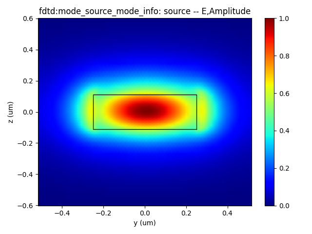
1.The electric intensity profile of the input fundamental TE mode and the transimission at different wavelengths.

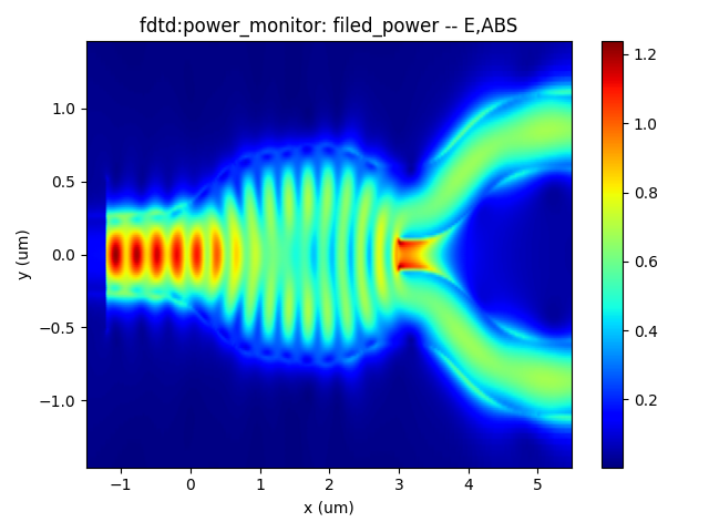
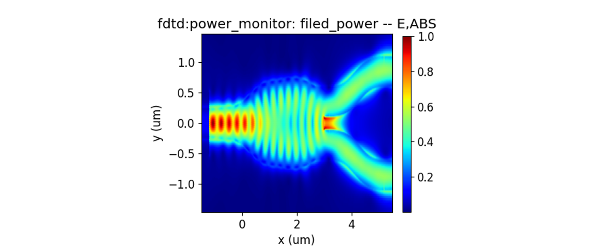
2.The z-normal E intensity of Y branch structure.

Above all,the insert loss of this Y branch device is about 0.628 dB at 1.55 micrometer wavelength.

Supplement

To view a function's definition and supported parameters or a parameter dictionary, you can right-click on its name and select "Go to Definition" or press "Ctrl" while left-clicking on its name to view its definition, showing the available parameters and their descriptions.